A tour of Maxima (with wxMaxima)
José A. Vallejo
Faculty of Science
State University of San Luis Potosí (México)
email: jvallejo@fc.uaslp.mx
URL: http://galia.fc.uaslp.mx/~jvallejo
Date: May 19 2019
ABSTRACT: In this document we try to illustrate the possibilities offered by the CAS (Computer Algebra System) Maxima, along the lines of the chapters "A Tour of Mathematica" that appeared in the printed versions of The Mathematica Book by Wolfram Research up to its 5th edition (2003). Although it is free software (as in 'freedom' and as in 'free beer'), the quality of Maxima is comparable to that of commercial programs such as Mathematica (TM) or Maple (TM). Its development began at the MIT (Massachusetts Institute of Technology) in the 60s, and it is nowadays active thanks to the dedicated work of a wide group of people around the world. Maxima admits many graphical interfaces (originally, it is invoked from the shell). The one we will use in this document is wxMaxima, although almost all of the results are independent of the interface (the only exception being the animations). This document has been created on a Linux platform running Slackware 14.2, with Maxima version 5.38.0 compiled against SBCL 1.3.5, and wxMaxima version 16.04.2.
Contents
REMARK: If the mathematical symbols are displayed in a sub-optimal way, please change the MathJax renderer of your browser: just click with the right button of the mouse on any of the equations below and, from the menu, select Math Settings - Math Renderer - SVG (for instance). The displayed output depends on which sets of fonts do you have installed in your system.
1 Basic Arithmetics
Arithmetics can be done in Maxima as in a calculator. For instance, we enter 13+11 and Maxima returns the result, 24.
| (%i1) | 13+11; |
However, in contrast to a calculator, Maxima can work with exact computations. Here we give the value of 3^100. The circumflex ^ is the symbol for the exponentiation.
| (%i2) | 3^100; |
The 'float' function gives approximate numerical results (by default, with 15 digits precision). The percent sign % is used to make reference to the last output (older results can be accesed trough %th(n)):
| (%i3) | float(%); |
Numerical results can be evaluated with any desired precision. The next command computes sqrt(10) with 50 digits, using "bfloat" (bigfloat number):
| (%i4) | bfloat(sqrt(10)),fpprec:50; |
Maxima can also work with complex numbers. Here we show the rectangular form of (3+4i)^10 computed in two alternative forms. The complex unit i is denoted %i (other important constants implemented by default are %e, %pi or %phi, notice that all of them begin with a % sign).
| (%i5) | (3+4·%i)^10,expand; |
| (%i6) | rectform((3+4·%i)^10); |
However, expansion is not done by default: in Maxima (3+4i)^10 is an expression in its own right!
| (%i7) | (3+4·%i)^10; |
More operations with complex numbers. The syntax is self-explaining, let us only remark that the colon ':' is used to assign values to variables (for instance, in the first line we assign the label z1 to the complex number 2+3i).
| (%i8) | z1:2+3·(%i); |
| (%i9) | z2:−1−5·%i; |
| (%i10) | realpart(z1); |
| (%i11) | imagpart(z2); |
| (%i12) | abs(z1+z2); |
| (%i13) | carg(1−1·%i); |
| (%i14) | expand(z1·z2); |
| (%i15) | z1/z2; |
As we are working symbolically, the result is not automatically simplified, we must explicitly ask for the simplification, in this case, to pass to the rectangular form:
| (%i16) | rectform(%); |
Of course, it is possible to go back and forth between the rectangular and polar forms:
| (%i17) | polarform(1−%i); |
| (%i18) | rectform(%); |
In these commands we have assigned a value to a variable through ':' as in z1:2+3*%i. Once that assignment is made, each time the symbol z1 appears Maxima will understand that it has the assigned value:
| (%i19) | z1; |
If we want to remove the assignment, we can use 'remvalue' (another, more drastic, option is to use 'kill')
| (%i20) | remvalue(z1); |
| (%i21) | z1; |
Lists are very basic constructs in Maxima. They are collections of elements enclosed between square brackets, and they can be assigned to a variable name like A, mylist, etc. For instance (the dollar sign $ is used here to prevent Maxima from writing the output of a command, which in this case is just a copy of the input):
| (%i22) | listA:[a,b,c,d]$ |
| (%i23) | listB:[1,2,3,4]$ |
Operations with lists are immediate:
| (%i24) | listA+listB; |
Also, most of the built-in functions of Maxima can operate directly on lists:
| (%i25) | listA^2; |
In many cases, it is necessary that the length of the lists be the same. Otherwise, Maxima will complain, as occurs if we try [1,2,3,4,5]*listB.
Functions of the argument x can be defined with the same syntax used in the blackboard, using ':=' as in the following example:
| (%i26) | f(x):=cos(x^2)+exp(sin(x)); |
and then can be evaluated:
| (%i27) | f(0); |
| (%i28) | 3·f(sqrt(%pi))+c; |
But Maxima offers another possibility for defining functions, called lambda functions, which are extremely powerful. The idea is to work with unnamed functions, as when one says 'consider the function that sends the variable argument u to the expression u^2+1'. This is done as follows:
| (%i29) | lambda([u],u^2+1); |
Obviously, this can't be used as it stands, but we can say something like 'map the function that squares its argument and sums 1 to the result' to every element in the list [1,2,3,4], like this:
| (%i30) | map(lambda([u],u^2+1),[1,2,3,4]); |
Isn't it magic?
Maxima can compute the numerical values of all the standard functions. As an example, consider the value at 14.5 of the Bessel function of the first kind J0:
| (%i31) | bessel_j(0,14.5); |
Next, we are going to compute a real root of J0(x) near x=14.5, with a 20-digits precision. We will use the 'mnewton' routine for this (as its name says, it uses the Newton method). As this routine is not loaded by default, we call it first. Also, notice the syntax: usually when we pass an argument to a function that works with equations, an expression 'expr' is taken as the equation 'expr=0'
| (%i32) | load("mnewton")$ |
| (%i33) | mnewton(bessel_j(0,x),x,14.5); |
Some functions, as 'mnewton', return their output as a list (in this case, a list with only one element which is in turn a list, [x=14.93091770848779]. That is called nested list). If we want to extract the result, we can do the following (another possibility is to use %[1](%) below, that is, [i] selects the i-th element of the list):
| (%i34) | solution:x,first(%); |
| (%i35) | solution; |
The reason for giving the output in the form of a list is that the command 'mnewton' has lots of options, some of them returning more onformation than just a value. Here, we solve a nonlinear system of equations:
| (%i36) | mnewton([2·3^u−v/u−5, u+2^v−4],[u,v],[2,2]); |
| (%i37) | usol:u,%[1]; |
| (%i38) | vsol:v,%th(2)[1]; |
Let us see the result:
| (%i39) | [usol,vsol]; |
2 Elementary Algebra and Calculus
Before we begin, let's clear all the variable assignments we have done up to now:
| (%i40) | kill(all); |
We can check that no assignment is stored by looking at the output of 'values', which keeps track of those of the form a:something
| (%i1) | values(); |
and by looking at the output of 'functions', which keeps track of the definitions of the form f(x):=
| (%i2) | functions(); |
Recall that Maxima can work not only with numbers, but also with algebraic expressions. Here we consider the expression 9(2+x)(x+y)+(x+y)^2:
| (%i3) | 9·(2+x)·(x+y)+(x+y)^2; |
The next command takes this expression, represented by %, raises it to the power of 3 and expands the result:
| (%i4) | expand(%^3); |
By factoring the output we obtain a much simpler form:
| (%i5) | factor(%); |
Factoring can be done in different numerical domains. By default, it is carried on inside the integers ring Z:
| (%i6) | factor(x^8−41·x^4+400); |
The following modification of this command executes the factorization in the Gaussian integers Z[i]:
| (%i7) | gfactor(x^8−41·x^4+400); |
It is possible to factor within other domains, it is enough to adjoin the appropriate roots (this is done by declaring the minimal polynomials that they satisfy). For instance, to factor in Z[sqrt(5)], we would do
| (%i8) | subst(a=sqrt(5),factor(x^8−41·x^4+400,a^2−5)); |
Due to their importance in many topics, Maxima has a good deal of functions related to polynomials:
| (%i9) | poly1:(x+1)^10; |
| (%i10) | poly2:x^3−5·x^2·y+3·x·y^2−7·y^3; |
| (%i11) | listofvars(%th(2)); |
| (%i12) | listofvars(%th(2)); |
The coefficients of a given polynomial can be extracted with 'coeff'. This function do not apply any simplification procedure (in contrast to 'apply', 'factor', and such):
| (%i13) | coeff(expand(poly1),x,5); |
| (%i14) | coeff(poly2,x); |
| (%i15) | coeff(poly2,y,2); |
The degree of a polynomial is extracted with 'hipow':
| (%i16) | hipow(expand(poly1),x); |
| (%i17) | hipow(poly2,y); |
The following command returns a list containing the coefficients of the polynomial poly1:
| (%i18) | coefficients1:makelist(coeff(expand(poly1),x,i),i,0,hipow(expand(poly1),x)); |
Thus, the coefficients of powers of x in poly2 are:
| (%i19) | coefficients2:makelist(coeff(poly2,x,i),i,0,hipow(poly2,x)); |
and those of y:
| (%i20) | coefficients3:makelist(coeff(poly2,y,i),i,0,hipow(poly2,y)); |
With 'nroots' we can know the number of real roots a polynomial posseses in a given interval:
| (%i21) | nroots(x^4+x^3−8·x^2−5·x+15,−10,10); |
In order to try to find those roots exactly, we can use 'solve':
| (%i22) | solve(x^4+x^3−8·x^2−5·x+15); |
In many cases, we will not be able to compute roots in an exact way. With 'realroots' we obtain rational approximations:
| (%i23) | realroots(x^4+x^3−8·x^2−5·x+15); |
Of course, in case the roots are integer or rational numbers, 'realroots' will give an exact answer:
| (%i24) | realroots(expand((1−x)^5·(2−x)^3·(3−x))); |
Multiplicities are stored in the variable 'multiplicities', as it should be:
| (%i25) | multiplicities; |
To compute real and complex roots in full generality, we can use 'allroots' (remark: when there are multiple roots, 'allroots' is not the best option. In those cases, it is better to try something like allroots(%i*p), if the polynomial has real coefficients):
| (%i26) | allroots((1+2·x)^3−(27/2)·(1 + x^5)); |
Polynomial division using Euclid's algorithm is done with the aid of 'divide'. The output is a list of the form [quotient, remainder], whose elements can be extracted individually:
| (%i27) | pol1:x^5 −7·x^4+3·x^2−5·x+9; |
| (%i28) | pol2:x^2+1; |
| (%i29) | divide(pol1,pol2); |
| (%i30) | quotient(pol1,pol2); |
| (%i31) | remainder(pol1,pol2); |
Maxima can also compute the greatest common divisor:
| (%i32) | gcd(pol1,pol2); |
| (%i33) | pol3:(x−1)·(x−2)^2·(x−3)^3; |
| (%i34) | pol4:(x−1)^2·(x−2)·(x−3)^4; |
| (%i35) | gcd(pol3,pol4); |
| (%i36) | factor(%); |
and the least common multiple:
| (%i37) | lcm(pol3,pol4); |
Here, we express (x+a+1)^4 as a polynomial in x by grouping powers in x:
| (%i38) | collectterms(expand((x+a+1)^4),x); |
Now, let's consider some elementary single-variable calculus operations. For instance, limits:
| (%i39) | limit(((a^(1/n)+b^(1/n))/2)^n,n,inf); |
| (%i40) | limit(log(n)/log(n+1),n,inf); |
| (%i41) | limit(n·(a^(1/n)−1),n,inf); |
The indeifnite integral of x^2 sin(x)^2:
| (%i42) | integrate(x^2·sin(x)^2,x); |
By differentiating the output, we should get the original integrand, albeit possibly in a different (but equivalent) form:
| (%i43) | diff(%,x); |
In order to see the equivalence of both expressions, we can resort to some simplifying commands that apply trigonometric relations. In the first place, we have 'trigsimp', that will try to write the given expression with the minimal number of trigonometric functions:
| (%i44) | trigsimp(%); |
THis result is expressed in terms of the cosine, and we want the sine. We then use 'trigexpand' to convert the cos(2x) term into factors containing sin(x) and cos(x):
| (%i45) | trigexpand(%); |
and, finally, we simplify again (Maxima prefers the sine over the cosine for this, hence the trick):
| (%i46) | trigsimp(%); |
Definite integration follows a similar syntax, adding the integration lower and upper limits, which can be infinite:
| (%i47) | integrate(exp(−x^2),x,0,inf); |
Numerical integration is also possible. Here we give the numerical value of int(sin(sinx)) between 0 and pi, using Romberg's method:
| (%i48) | romberg(sin(sin(x)),x,0,%pi); |
The 'diff' command admits several arguments to differentiate functions with any number of variables an arbitrary number of times. The next command also illustrates the fact that the apostrophe ' delays the evaluation of the function that it precedes:
| (%i49) | k(x,y,z):=(x^2+y^4+1)·exp(z^2/y); |
| (%i50) | 'diff(k,x,2)=diff(k(x,y,z),x,2); |
| (%i51) | 'diff(k,z,2)=diff(k(x,y,z),z,2); |
The following command computes the Taylor expansion of the sin(x) function around x=0, up to degree 6:
| (%i52) | taylor(sin(x),x,0,6); |
Maxima is able to compute the Taylor development of a purely symbolic function. However, as the values of f are unknown, its derivatives are also unknown and must be declared in some way. A possibility is to use 'gradef', but a much better solution is to consider the package 'pdiff', which establishes a positional notation for the derivatives: given f=f(x), the n-th derivative with respect to x will be denoted f_(n)(x). If f=f(x,y) is a fucntion of two variables, f_(2,1)(x,y) will denote a third derivative of f, twice with respect to x and once with respect to y, etc. Thus, consider
| (%i53) | g(x,h):=(f(x+h)−f(x−h))/(2·h); |
| (%i54) | load(pdiff)$ |
| (%i55) | taylor(g(x,h),h,0,6); |
The output of the command 'taylor' is a series, and as such it has properties which are different from those of a polynomial. If we want to use the 6th degree polynomial above, we need to make a truncation:
| (%i56) | define(T(x,h),trunc(%)); |
| (%i57) | T(x,0.1); |
Finally, multiple integration works as one would expect:
| (%i58) | 'integrate('integrate((x^2+4·y),x,11,14),y,7,10) = integrate(integrate(x^2+4·y,x,11,14),y,7,10); |
3 Elementary Number Theory
Maxima knows about the Golden Number (or Divine Proportion, Golden Constant, etc.)
| (%i59) | %phi,bfloat; |
However, Maxima does not establish its algebraic properties by default. We can do it by ourselves, declaring %phi as the only positive root of the polynomial x^2-x-1. The command 'tellrat' adds a number to the ring of algebraic integers already known by Maxima:
| (%i60) | tellrat(%phi^2−%phi−1); |
| (%i61) | algebraic:true; |
| (%i62) | is(equal(%phi^3,(%phi+1)/(%phi−1))); |
| (%i63) | is(equal(%phi,(1+sqrt(5))/2)); |
Here is the continued fractions expansion of %phi (of length 3):
| (%i64) | ratprint:false$ |
| (%i65) | cf(ev(%phi,numer)); |
Notice the length of the period. Things look better if we use a rational form for %phi:
| (%i66) | cf((1+sqrt(5))/2),cflength:2; |
| (%i67) | cfdisrep(%); |
Fibonacci numbers can be expressed in terms of %phi, a fact also implemented in stock Maxima:
| (%i68) | fibtophi(fib (n)); |
It is also useful to have available commands for dealing with prime numbers:
| (%i69) | next_prime(23648357231245341550071721324); |
We can determine whether a number is prime or not by applying some primality test. For integres greater than 341550071728321, probabilistic algorithms (such as Miller-Rabin and Lucas) are used:
| (%i70) | primep(23648357231245341550071721453); |
The number of pseudo-primality tests to be run is given by the value of the variable 'primep_number_of_tests', here is its default value:
| (%i71) | primep_number_of_tests; |
Maxima uses exact arithmetic when dealing with integers. The function 'factor', for instance, gives the prime factors decomposition of an integer:
| (%i72) | factor(70612139395722186); |
It is possible to get a list with the prime factors and their exponents for later use:
| (%i73) | ifactors(70612139395722186); |
It is known that the number ϕ(n)/n (where ϕ is Euler's totient function) approximates the probability that a positive integer chosen at random, be coprime with p1 , . . . , pk , where n = p1^e1 · · · pk^ek is the prime factorization of n. One could write first a program that selects m random numbers between 1 and 100m. The 'block' environment offers the possibility of defining some local variables (in this case, s and N) whose previous values will be stored and then erased, after exiting the block, they will be restored. Then, we can write a sequence of instructions (separated by commas) using the usual programming structures for loops, stop conditions, etc. The last instruction determines the output. In this regard, the following very simple function 'numgen' clearly illustrates these ideas:
| (%i74) |
numgen(m):=block([s,N], N:100·m, for j:1 thru m do s[j]:random(N), makelist(s[j],j,1,m) )$ |
| (%i75) | numgen(10); |
For a list of such numbers, we can complete the fraction of those coprime with n (notice the appearance of the function 'gcd' for this):
<| (%i76) |
P(m,n):=block([tmp,N], N:numgen(m), for k:1 thru m do t[k]:gcd(n,N[k]), tmp:makelist(t[k],k,1,m), length(sublist_indices(tmp,lambda([x],x='1)))/m )$ |
Also notice the use of lambda functions here. Finally, we can check that P (m, n), for large values of m, approaches ϕ(n)/n:
| (%i77) | P(5500,92),numer; |
| (%i78) | totient(92)/92,numer; |
4 Graphics
There are two options available to create graphics in Maxima: the set of functions 'plot2d', 'plot3d' and the more powerful (and complex) 'draw2d', 'draw3d'. In each case, there exists a wrapper for wxMaxima that can be called just adding the prefix 'wx' to each command, resulting in graphics embedded into the wxMaxima worksheet (if only, say, plot3d is used, the graphics will appear in a separate window). Maxima uses the external grapher Gnuplot for these tasks, so it must be previously installed in your system.
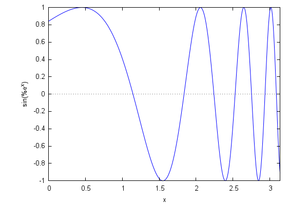
Here is a simple drawing: the graph of the function sin(exp(x)) with x running in [0,pi]:
| (%i79) | wxplot2d(sin(exp(x)),[x,0,%pi]); |
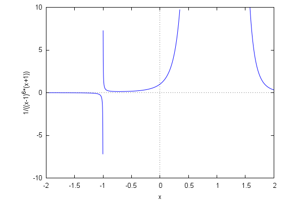
Maxima tries to define a range of values for the y variable which are appropriate for the function at hand, but sometimes we need to make some adjustments. Consider, for example, the case of the function 1/(x+1)(x-1)^6:
| (%i80) | wxplot2d(1/(x+1)·(x−1)^6,[x,−2,2]); |
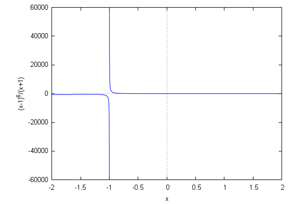
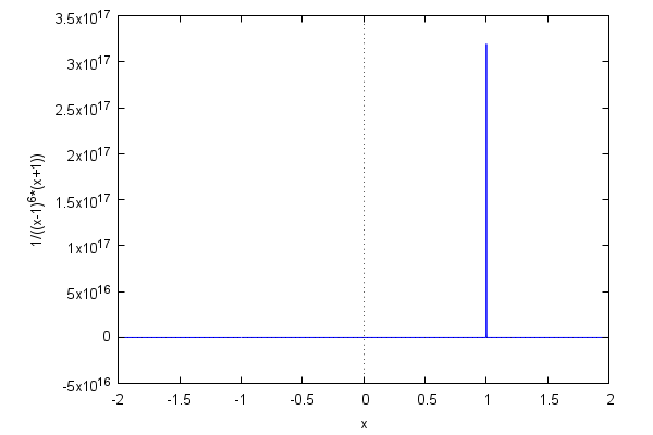
The default range reflects the existence of a pole at x=-1 of order 1. However, the function has another pole at x=1 (of order 6) which can be made apparent by writing the function in an equivalent form:
| (%i81) | wxplot2d(1/(x+1)/(x−1)^6,[x,−2,2]); |
It is clear that no single range of values will be adequate to accurately represent two poles of such disparate orders. A little bit of trial and error applied to [y,ymin,ymax] leads to a more or less satisfying compromise:
| (%i82) | wxplot2d(1/(x+1)/(x−1)^6,[x,−2,2],[y,−10,10]); |
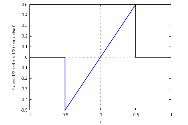
It is possible to define and draw piecewise-defined functions:
| (%i83) | s(x,L):=if (x>=−L/2 and x<L/2) then x else 0$ |
| (%i84) | L:1$ |
| (%i85) | wxplot2d(s(x,L),[x,−L,L],[style,[lines,2]]); |
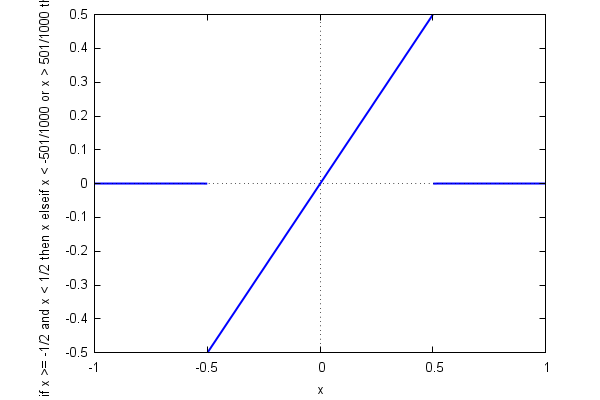
If we do not want the vertical lines that Gnuplot introduces in order to 'complete' the graph of the function, we can employ a little trick:
| (%i86) | t(x,L):=if (x>=−L/2 and x<L/2) then x elseif (x<−L/2−10^(−3) or x>L/2+10^(−3)) then 0$ |
| (%i87) | wxplot2d(t(x,L),[x,−L,L],[style,[lines,2]]); |
Here is a representation of the complex roots of z^n=1 in the plane:
| (%i88) | n:300$ |
| (%i89) | soln:map(lambda([x],rhs(x)),allroots(z^n−1))$ |
| (%i90) | pnts:map(lambda([x],[realpart(x),imagpart(x)]),soln)$ |
| (%i91) | wxplot2d([discrete,pnts],[style,[points,0.25,2,1]],same_xy); |
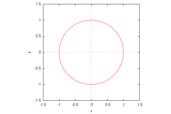
Notice the 'same_xy' option here! It tells Maxima to use the same scale for the x and y axes: Maxima uses a 600x400 default canvas, so the original scales are in a 3:2 proportion, which would lead to a distorted graphics.
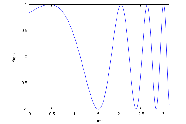
We have already remarked that Maxima uses an external grapher, Gnuplot, which posseses many options to adjust the graphical output. Here are some of them:
| (%i92) |
wxplot2d( sin(exp(x)),[x,0,%pi], [xlabel,"Time"],[ylabel,"Signal"], [gnuplot_preamble,"set grid; set xtics 0.5; set ytics 0.5"] ); |
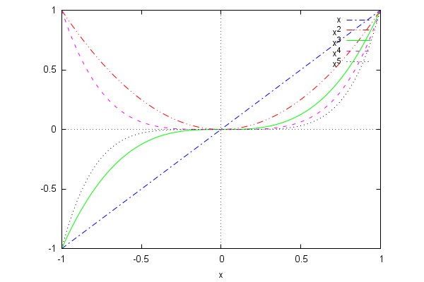
Gnuplot supports many types of lines. Their appearance is controlled by the options 'linetype' and 'dashtype', which are called using 'gnuplot_preamble', an instruction that allows us to use the Gnuplot syntax directly inside Maxima:
| (%i93) |
wxplot2d( makelist(x^k,k,1,5), [x,−1,1], [gnuplot_preamble, "set for [i=1:5] linetype i dashtype i+3"] ); |
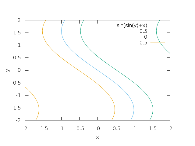
The contour diagram for the function sin(x+sin(y)). The option 'set cntrparam levels' determines the number of level sets to be shown:
| (%i94) | wxcontour_plot(sin(x+sin(y)),[x,−2,2],[y,−2,2],[gnuplot_preamble,"set cntrparam levels 3"]); |
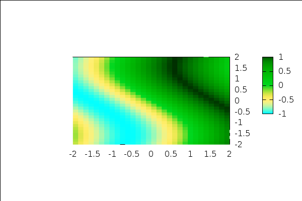
This is better seen with a color code. Lighter areas belong to lower level sets:
| (%i95) |
wxplot3d( sin(x+sin(y)),[x,−2,2],[y,−2,2], [mesh_lines_color,false],[grid,100,100], [elevation,0],[azimuth,0],[zlabel,""] ); |
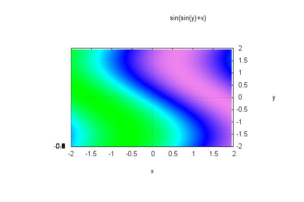
The z axis marks accumulate creating a disappointing spot (the graphics is obtained by projecting the surface from above onto the plane z=0). A possibility for obtaining a clearer drawing consists in using 'draw3d' (previously loading the package 'draw'):
| (%i96) | with_stdout("/dev/null",load(draw))$ |
| (%i97) |
wxdraw3d( surface_hide=true, view=[0,360],zaxis=false,zlabel="",ztics=none, enhanced3d=true,palette=[15,−8,−5],cbtics=0.5, explicit(sin(x+sin(y)),x,−2,2,y,−2,2) ); |
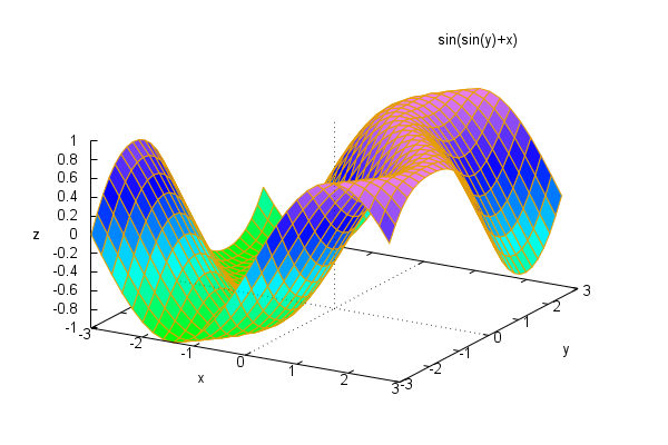
Here is a 3D representation of the same function (all of the following examples are better visualized if the instructions 'plot3d' and 'draw3d' are used, the reader can then click on the external Gnuplot window moving the mouse to rotate the graphics):
| (%i98) | wxplot3d(sin(x+sin(y)),[x,−3,3],[y,−3,3]); |
The 'plot3d' command works good with explicit surfaces of the form z=f(x,y), but if we need to create graphics for parametric curves or surfaces, it is better to use the several variants of 'draw' (in fact, 'draw' supports explicit, implicit as well as parametric drawings):
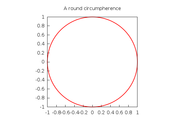
As an example, let us see how to represent a circumpherence explicitly, in parametric form and implicitly. We will take the opportunity to show other options, such as line color, line width, titles, etc.
| (%i99) |
wxdraw2d( explicit(sqrt(1−x^2),x,−1,1), explicit(−sqrt(1−x^2),x,−1,1), title="A round circumpherence", proportional_axes=xy ); |
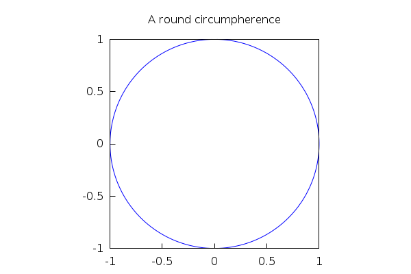
Notice the use of 'proportional_axes=xy'! By default, draw uses a 600x400 canvas, so the plot of a circumpherence will appear distorted if we do not use that option (which has the effect of using the same scale in both axes, not the 3/2 proportion). It is the analog of the 'same_xy' option that we used in plot2d.
| (%i100) |
wxdraw2d( line_width=2, color=red, parametric(cos(t),sin(t),t,0,2·%pi), title="A round circumpherence", proportional_axes=xy ); |
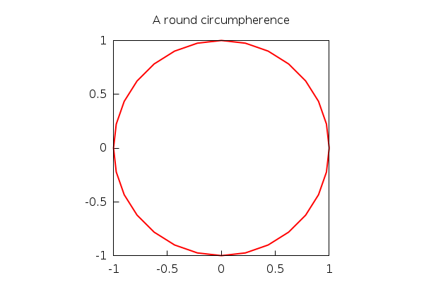
Here, we can see that the number of default 'ticks' used to construct the parametric curve is not enough. Maxima uses a default of 30 subdivisions of the interval, in this case [0,2pi], which gives the impression of a polygon, rather than a smooth curve. We can fix this by increasing the number of subdivisions with 'nticks':
| (%i101) |
wxdraw2d( line_width=2, color=red, nticks=180, parametric(cos(t),sin(t),t,0,2·%pi), title="A round circumpherence", proportional_axes=xy ); |
Finally, an implicit drawing:
| (%i102) |
wxdraw2d( line_width=2, color=orange, implicit(x^2+y^2=1,x,−1,1,y,−1,1), title="The third circumpherence", proportional_axes=xy ); |
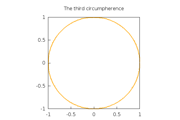
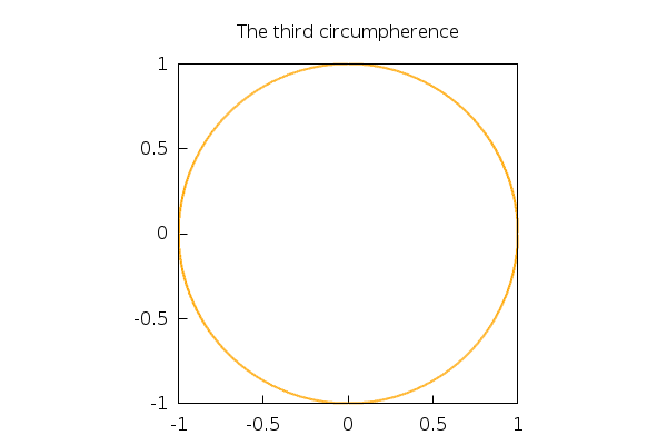
Implicit drawings require a lot of computational work, and should be avoided whenever possible. We can increase the quality of the output by means of 'ip_grid' (that will also increase the timing!)
| (%i103) |
wxdraw2d( line_width=2, color=orange, ip_grid=[100,100], implicit(x^2+y^2=1,x,−1,1,y,−1,1), title="The third circumpherence", proportional_axes=xy ); |
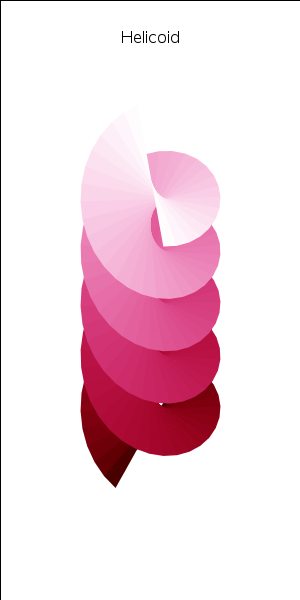
Next, we generate a parametric surface, with the points x,y,z on the surface gievn as functions of the parameters u,v. It is important to notice the use of the 'wxplot_size' variable to match the size of the Gnuplot drawing with the size of the wxMaxima canvas in which we will draw it:
| (%i104) |
wxdraw3d( title="Helicoid", axis_3d=false,xtics='none,ytics='none,ztics='none, xu_grid=75,yv_grid=35,dimensions=[300,600], surface_hide=true, enhanced3d=true,palette=[8,4,3],colorbox=false, parametric_surface(v·sin(u),v·cos(u),u/3,u,0,15,v,−1,1) ),wxplot_size=[300,600]; |
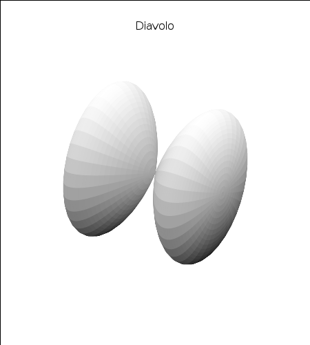
Here is a more complex parametric surface:
<| (%i105) |
wxdraw3d( title="Diavolo", axis_3d=false,xtics='none,ytics='none,ztics='none, xu_grid=75,yv_grid=35,dimensions=[450,500], surface_hide=true, enhanced3d=true,palette=gray,colorbox=false, parametric_surface(sin(u),sin(2·u)·sin(v),sin(2·u)·cos(v),u,−%pi/2,%pi/2,v,0,2·%pi) ),wxplot_size=[450,500]; |
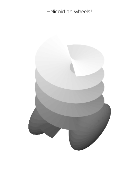
It is possible to combine several plots in one scene:
| (%i106) |
wxdraw3d( title="Helicoid on wheels!", axis_3d=false,xtics='none,ytics='none,ztics='none, xu_grid=75,yv_grid=35,dimensions=[450,600], surface_hide=true, enhanced3d=true,palette=gray,colorbox=false, parametric_surface(v·sin(u),v·cos(u),u/3,u,0,15,v,−1,1), parametric_surface(sin(u),sin(2·u)·sin(v),sin(2·u)·cos(v),u,−%pi/2,%pi/2,v,0,2·%pi) ),wxplot_size=[450,600]; |
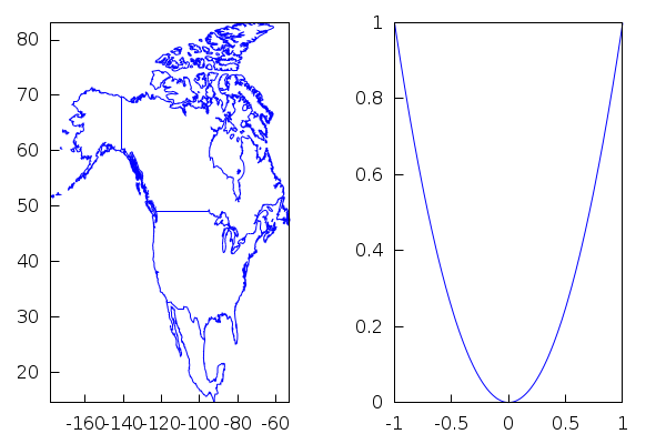
The 'draw' package can call a little library called 'worldmap' which contains cartographical data:
| (%i107) | load(worldmap)$ |
| (%i108) | comp1:gr2d(geomap([United_States,Canada,Mexico]))$ |
| (%i109) | comp2:gr2d(color=blue,explicit(x^2,x,−1,1))$ |
The next commands generate a two-scene graphics (better seen in an independent window, just replace 'wxdraw' below by 'draw'):
| (%i110) | wxdraw( columns=2, dimensions=[1000,500], comp1,comp2); |
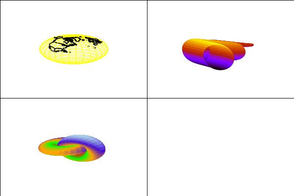
Let's see how to represent several 3D graphics together:
| (%i111) |
escena1:gr3d( surface_hide=true,axis_3d=false,xtics='none,ytics='none,ztics='none,xlabel="",ylabel="",zlabel="", color=yellow, parametric_surface(cos(phi·%pi/180)·cos(theta·%pi/180),cos(phi·%pi/180)·sin(theta·%pi/180),sin(phi·%pi/180),theta,−180,180,phi,−90,90), color=black, line_width=2, geomap([North_America,Europe]) )$ |
| (%i112) |
escena2:gr3d( axis_3d=false,xtics='none,ytics='none,ztics='none,xlabel="",ylabel="", enhanced3d = true,palette=color,colorbox=false, xu_grid = 50, tube(cos(a),a,0,cos(a/10)^2,a,0,4·%pi) )$ |
| (%i113) |
escena3:gr3d( enhanced3d=sin(u)+cos(v),palette=["#ff0000",green,orange,"#450cd2",light_blue], colorbox=false, dimensions=50·[15,15], axis_3d=false,xtics='none,ytics='none,ztics='none,xlabel="",ylabel="", parametric_surface(cos(u)+.5·cos(u)·cos(v),sin(u)+.5·sin(u)·cos(v),.5·sin(v),u,−%pi,%pi,v,−%pi,%pi), parametric_surface(1+cos(u)+.5·cos(u)·cos(v),.5·sin(v),sin(u)+.5·sin(u)·cos(v),u,−%pi,%pi,v,−%pi,%pi) )$ |
| (%i114) | wxdraw(columns=2,escena1,escena2,escena3); |
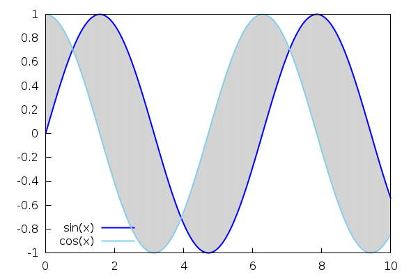
With 'draw' we can also create advanced 2D graphics. For instance, we can shadow the area between curves with 'filled_func'. Many more options can be found in the documentation.
| (%i115) |
wxdraw2d( filled_func=sin(x),fill_color=light−gray, explicit(cos(x),x,0,10), filled_func=false,color=blue,line_width=2,key="sin(x)", explicit(sin(x),x,0,10), color=skyblue,line_width=2,key="cos(x)", explicit(cos(x),x,0,10), user_preamble="set key left bottom" ); |
5 Data fitting
| (%i116) | kill(all); |
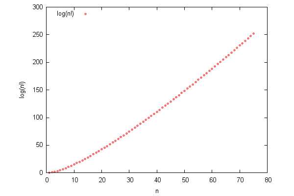
We have already had occasion to work with lists before. The following command creates a list containing the first 75 factorials (we chose not to show it with the symbol $ at the end of the command):
| (%i1) | Lista:makelist(n!,n,1,75)$ |
Next, we take the logarithm of each element in the list and numerically evaluate the result. Most of Maxima built-in functions, like 'log' have the property of being 'listable', so they are applied individually to each element:
| (%i2) | lista:log(%),bfloat$ |
Individual elements of the list a:[a_1,...,a_n] can be extracted by specifying their indices, as in a[i]. Thus,
| (%i3) | Lista[4]; |
| (%i4) | lista[4]; |
Let's check that the first number Lista[4] is the exponential of the second lista[4] (for this, we must express the floating numbers returned by the exponential as rationals. This behavior is controlled by the environment variable 'bftorat'; the other variable 'ratprint', when set to 'false', avoids that some message telling that such or such number was converted to rational be emitted):
| (%i5) | rat(%e^lista[4]),bftorat:true,ratprint:false; |
Now we generate a graphics representing the entries in lista against those in Lista. The fact that the points seem to distribute asymptotically near a straight line is a consequence of a mathematical result known as Stirling's formula: log(n!) behaves as nlogn, for big values of n.
| (%i6) | P:makelist([k,lista[k]],k,1,length(lista))$ |
| (%i7) |
wxplot2d( [discrete,P], [style,[points,1]],[point_type,circle],[color,red], [xlabel,"n"],[ylabel,"log(n!)"], [legend, "log(n!)"], [gnuplot_preamble,"set key left top"] ); |
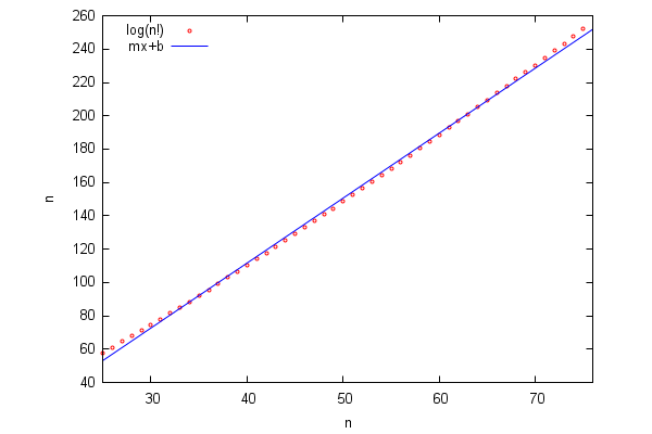
Maxima has a function to fit data using the least squares technique, not surprisingly contained in the package 'lsquares'.
| (%i8) | load(lsquares)$ |
As Stirling's formula is asymptotic, we discard the first 24 values (which would lead to a distorted fitting)
| (%i9) | Q:lastn(P,51)$ |
First, our list of points must be converted into a matrix:
| (%i10) | data:funmake('matrix,Q)$ |
Then, the function "lsquares_estimates" fits the data in that matrix (whose first column is interpreted as containing the 'x' coordinates, while the second contains the 'y' ones) to a straight line y=mx+b, and gives us the values of the coefficients m,b:
| (%i11) | lsquares_estimates(data,[x,y],y=m·x+b,[m,b]),numer; |
| (%i12) | m:rhs(%[1][1]); |
| (%i13) | b:rhs((%th(2))[1][2]); |
Now we can plot the data and the fitting curve in the same graphics:
| (%i14) |
wxplot2d( [[discrete,Q],m·x+b],[x,25,25 + length(Q)], [style,[points,1],lines],[point_type,circle],[color,red,blue], [xlabel,"n"],[ylabel,"n"], [legend, "log(n!)", "mx+b"], [gnuplot_preamble,"set key left top"] ); |
6 Linear Algebra
| (%i15) | kill(all); |
Let us start by defining a matrix to play with:
| (%i1) | C:matrix([1,2,3,4],[5,6,7,8],[9,10,11,12],[13,14,15,16]); |
Here we compute a basis of the null subspace (the kernel) of the linear mapping determined by C:
| (%i2) | nullspace(C); |
The result is given in the form of column vectors (neither matrices nor lists). Hence, the procedure to extract the basis vectors of Ker(C) is a little bit elaborated:
| (%i3) | transpose(args(%)[1])[1]; |
| (%i4) | map(transpose,args(%th(2)))[2][1]; |
The dimension of ker(C) is directly given by 'nullity;:
| (%i5) | nullity(C); |
Of course, we can also compute a basis of the column subspace (image subspace, Im(C))
| (%i6) | B1:columnspace(C); |
and the corresponding dimension:
| (%i7) | rank(C); |
In the following command, we compute a basis of the orthogonal complement to Im(C):
| (%i8) | B2:apply('orthogonal_complement,args(columnspace(C))); |
We can check that these vectors and those in the basis B2 (of columnspace(C)) are orthogonal. Notice here how to define a matrix from a pre-existing function of two indexes as arguments:
| (%i9) | p[i,j]:=dotproduct(args(B1)[i],args(B2)[j])$ |
| (%i10) | genmatrix(p,2,2); |
Continuing with this idea, next we generate a 3x3 matrix whose (i,j) coefficient is 1/(i+j+1):
| (%i11) | kill(b)$ |
| (%i12) | b[i,j]:=1/(i+j+1); |
| (%i13) | M:genmatrix(b,3,3); |
The inverse of M is
| (%i14) | invert(M); |
Multiplying the inverse by the original matrix we get the identity matrix (the usual . , not * , is used in Maxima to denote the matrix product):
| (%i15) | %.M; |
The following command outputs a new matrix, with a modified diagonal. It is important to pay attention to the way the 3x3 identity matrix is written:
| (%i16) | M−x·ident(3); |
The determinant of this new matrix is precisely the characteristic polynomial of the original matrix:
| (%i17) | ratsimp(determinant(%)); |
| (%i18) | expand(%); |
The same computation can be done directly with the function 'charpoly':
| (%i19) | expand(charpoly(M,x)); |
With 'eigenvalues', we can find the numerical values of the eigenvalues of M (what a surprise!). Their multiplicities are also given inside the output, as a separate list:
| (%i20) | eigenvalues(M),numer; |
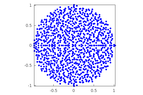
The following commands generate a (pseudo) random matrix 1000x1000 (with real coefficients normally distributed around the mean 0 with variance 1):
| (%i21) | load(distrib)$ |
| (%i22) | P:apply(matrix,makelist(random_normal(0,1,1000),i,1,1000))/sqrt(1000)$ |
In order to compute the eigenvalues of such a matrix, highly specialized routines, which can be found in the package 'lapack', must be used. In this case, we will need the command 'dgeev'.
| (%i23) | with_stdout("/dev/null",load("lapack"))$ |
| (%i24) | dgeev(%th(2))$; |
Let us represent the output in the complex plane, to visualize the distribution of the eigenvalues:
| (%i25) | preal:realpart((%)[1])$ |
| (%i26) | pimag:imagpart((%th(2))[1])$ |
The result is a numerical proof of Girko's Circular Law:
| (%i27) | wxdraw2d(proportional_axes=xy,point_type=filled_circle,point_size=1, points(preal,pimag),xtics=0.5); |
Symbolic matrices are also valid. In this example, we compute the eigenvalues and eigenvectors of a matrix of indeterminate coefficients:
| (%i28) | eigenvectors(matrix([u,v],[−v,2·u])); |
Some particular matrices are already built-in, like Vandermonde matrices:
| (%i29) | vandermonde_matrix([x,y,z]); |
The determinant of such a matrix is computed by means of the classical formula:
| (%i30) | factor(determinant(%)); |
Maxima can compute the Jordan normal form of a matrix directly. The related functions are contained in the package 'diag':
| (%i31) | load(diag)$ |
In this case, we have a diagonalizable matrix:
| (%i32) | M: matrix( [18,−51,27,−15], [8,−24,14,−8], [15,−48,28,−15], [15,−47,25,−12] ); |
| (%i33) | jordan(M); |
The output of the command 'jordan' is a list of eigenvalues with their multiplicities (or, in general, Jordan blocks). To display the matrix proper, we do
| (%i34) | dispJordan(%); |
Let us consider the general case. Again, notice that the output of the functions is given in the form of lists:
| (%i35) | N:matrix([2,0,0,1,0,0,1,0], [1,2,0,0,0,0,0,0], [−4,1,2,0,0,0,0,0], [2,0,0,2,0,0,0,0], [−7,2,0,0,2,0,0,0], [9,0,−2,0,1,2,0,0], [−34,7,1,−2,−1,1,2,0], [15,−17,−16,3,9,−2,0,3]); |
| (%i36) | jordan(N); |
| (%i37) | dispJordan(%); |
Functions of matrices can be computed with the aid of the command 'mat_function', also contained in 'diag':
| (%i38) | T:matrix([0,1,0,0],[0,0,0,2·c],[0,0,0,1],[0,−2·c,3·c^2,0]); |
| (%i39) | mat_function(exp,t·T); |
| (%i40) | expand(trigrat(%)); |
The Gram-Schmidt orthonormalization process with respect to the Euclidean canonical product in R^n (stored in the variable 'innerproduct') is carried on with the command 'gramschmidt', contained in the package 'eigen':
| (%i41) | load(eigen)$ |
| (%i42) | gramschmidt([[1,2,1,3],[2,2,2,2],[1,−1,1,−1],[3,4,3,5]]); |
Let us check that the resulting vectors form an orthogonal system:
| (%i43) | map(innerproduct,[%[1],%[2],%[3]],[%[2],%[3],%[1]]); |
It is possible to define the scalar product to be used, and to pass it as an argument to 'gramschmidt'. In the following commands, we use this idea to construct the Legendre polynomials normalized so as to make their leading coefficient equal to 1:
| (%i44) | prodesc(f,g):=integrate(f·g,u,−1,1)$ |
| (%i45) | gramschmidt([[1],[u],[u^2],[u^3],[u^4],[u^5]],prodesc); |
| (%i46) | expand(%); |
A quick check:
| (%i47) | prodesc(%[3],%[5]); |
7 Differential Equations
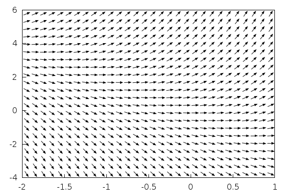
Maxima can represent the slope field (isoclines) of a differential equation without problems. Here, we use the equation dy/dx=2x+y with x running in [-2,1] and y in [-4,6]:
| (%i48) | load(drawdf)$ |
| (%i49) | wxdrawdf(2·x+y,[x,−2,1],[y,−4,6]); |
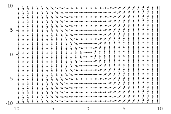
The same command 'drawdf' (or its wxMaxima version) allows us to study the phase diagram of a first-order system (equivalently, a second-order differential equation), in this example
du/dt=v^2
du/dt=u^3
| (%i50) | wxdrawdf([v^2,u^3],[u,v]); |
Problems involving initial conditions can be solved, too. The problem dy/dx=x+y with y(0)=2 uses the commands 'ode2' (for solving the equation) and 'ic1' (for applying the initial conditions):
| (%i51) | eq1:'diff(y,x)=x+y; |
| (%i52) | ode2(%,y,x); |
| (%i53) | ic1(%,x=0,y=2); |
There is a similar command, 'ic2', to deal with second-order equations:
| (%i54) | eq2:'diff(y,x,2)−y=0; |
| (%i55) | ode2(eq2,y,x); |
| (%i56) | ic2(%,x=0,y=1,'diff(y,x)=%pi); |
Boundary-value problems for second-order differential equations are the target of 'bc2'. For instance, d²y/dx²+y=0 with conditions y(0)=0,y(pi)=1, has no solution:
| (%i57) | eq3:'diff(y,x,2)+y=0; |
| (%i58) | ode2(eq3,y,x); |
| (%i59) | bc2(%,x=0,y=0,x=%pi,y=1); |
The same equation with conditions y(0)=0,y(pi/2)=1 has a unique solution:
| (%i60) | bc2(%th(2),x=0,y=0,x=%pi/2,y=1); |
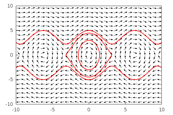
Here is the phase diagram of a pendulum with the trajectories through some points selected with the function 'solns_at':
| (%i61) | wxdrawdf([y,−5·sin(x)],line_width=2,solns_at([0,−5],[0,−3],[0,5],[%pi−0.0001,0])); |
Ordinary differential equations with parameters are admissible, too. Here we compute the solution of y''(x)-ky(x)=1, assuming k>0:
| (%i62) | assume(0<k); |
| (%i63) | ode2('diff(y,x,2)−k·y=1,y,x); |
Had we not used the assumption on k above, Maxima would ask us about the sign of k. The form of the solution depends crucially on the sign of k, as we can check:
| (%i64) | forget(0<k); |
| (%i65) | assume(k<0); |
| (%i66) | ode2('diff(y,x,2)−k·y=1,y,x); |
| (%i67) | forget(k<0); |
| (%i68) | assume(equal(k,0)); |
| (%i69) | ode2('diff(y,x,2)−k·y=1,y,x); |
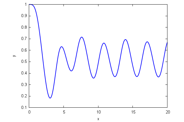
To numerically solve a second-order differential equation, Maxima offers the function 'rk', which implements the Runge-Kutta method of order four. However, this function only accepts first-order differential equations or systems, so in order to solve an equation like y''(x)+sin(x)^2 y'(x)+y(x)=cos(x)^2, with initial conditions y(0)=1, y'(0)=0, we must write it as a first-order system first. The procedure is standard: introduce an auxiliary function u(x) and write
y'(x)=u(x)
u'(x)=-sin(x)^2 u(x)-y(x)+cos(x)^2
Now we can apply 'rk'. For instance, to compute y(x) with x running in [0,20]:
| (%i70) | rk([u,−sin(x)^2·u−y+cos(x)^2],[y,u],[1,0],[x,0,20,0.1])$ |
The result is a list of sublists having the form [xi,yi,ui]. We are interested in the graphical representation of the solution y(x), that is, the first two elements of each sublist, that we can extract as follows:
| (%i71) | datos:rk([u,−sin(x)^2·u−y+cos(x)^2],[y,u],[1,0],[x,0,20,0.1])$ |
| (%i72) | puntos:makelist([datos[i][1],datos[i][2]],i,1,length(datos))$ |
| (%i73) | wxplot2d([discrete,puntos],[x,0,20],[style,[lines,2]]); |
8 Bessel Functions
| (%i74) | kill(all); |
Bessel functions are implemented in stock Maxima, but they are treated symbolically (that is, they are not evaluated by default) except by certain functions like 'specint'. This is the same that happens when you write
| (%i1) | (a+b)^3; |
Probably you would expect to see a^3+3ba^2+3b^2a+b^3, but this is not the output, because Maxima treats symbolic expressions in a symbolic manner, so it sees (a+b)^3 as a whole. If you want the expansion of this expression, you have to ask for it explicitly:
| (%i2) | expand((a+b)^3); |
Well, as mentioned, the same happens in the case of Bessel functions:
| (%i3) | bessel_j(0,2); |
If we want a numerical result, we must ask for it:
| (%i4) | bessel_j(0,2),numer; |
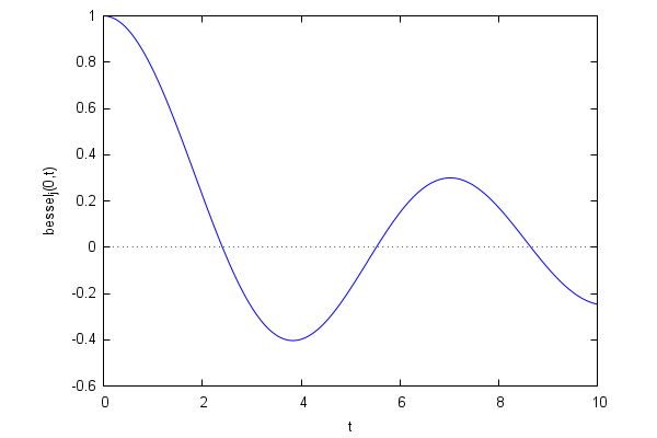
To draw the Bessel functions, we can use the evluation operator on functions, given by '' (two simple apostrophes). This forces the function to evaluate the result, not just to store it. Now everything is easy:
| (%i5) | wxplot2d(''bessel_j(0,t),[t,0,10]); |
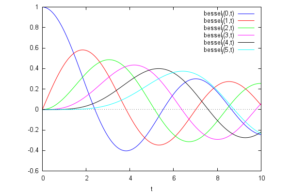
The graphics appearing in every textbook:
| (%i6) | wxplot2d( makelist(''bessel_j(n,t),n,0,5),[t,0,10] ); |
We could look for roots in an interval [a,b] with the command 'find_root' but we must keep on mind that the computation is stopped once the first root is found, so it is not possible to apply it to list all the roots in a big interval such as [0,10]. For instance, in the case of J0 we could do something like
| (%i7) | find_root(''bessel_j(0,t),t,0,4); |
| (%i8) | find_root(''bessel_j(0,t),t,4,7); |
| (%i9) | find_root(''bessel_j(0,t),t,7,10); |
The calculations can be simplified if we recall the Sturm theory, which says that the distance between two consecutive zeros tends to pi. Thus, we can look for zeros in an interval by dividing it into segments of length close to pi. In the case of the zeros of J0 over the interval [0,10] we would do
| (%i10) | makelist( find_root(''bessel_j(0,t),t,k·%pi,(k+1)·%pi),k,0,2 ); |
A simple function for computing the zeros of J0 in [a,b] can be written along these lines:
| (%i11) | cerosj0(a,b):=block([m], m:floor(b/%pi), makelist( find_root(''bessel_j(0,t),t,a+k·%pi,a+(k+1)·%pi),k,0,m−1) )$ |
so the above example would read now
| (%i12) | cerosj0(0,10); |
Our little function can answer questions such as: what are the first 40 zeros of J0? The result is given in the form of a list, named 'first40' so we can use it later:
| (%i13) | first40:cerosj0(0,40·%pi); |
Of course, we can numerically prove the Sturm prediction stating that the interval between consecutive roots tends to pi:
| (%i14) | makelist( first40[k+1]−first40[k],k,1,39 ); |
As an easy exercise, the reader will have no problem in adapting the preceding computations to the case of other Bessel functions J_nu and Y_nu.
9 Animations
Maxima, when used in conjunction with its interface wxMaxima, allows the user to create very basic animations depending on a parameter (the 'slider'). Next, we show an illustration of the tangent line to a function at a point (to see the animation, just click on the graphics with the left button of the mouse, or with the right one and select "Start Animation"):
| (%i15) | f(x):=sin(x)$ |
| (%i16) | tang(a,x):=f(a)+cos(a)·(x−a)$ |
| (%i17) |
with_slider_draw( a,makelist(%pi·i/6,i,0,12), line_width=1,color=blue,key="f(x)", explicit(f(x),x,0,2·%pi), line_width=2,color=green,key="tangent", explicit(tang(a,x),x,a−1/sqrt(1+cos(a)^2),a+1/sqrt(1+cos(a)^2)), point_size=1,color=red,point_type=filled_circle,key="", points([[a,f(a)]]), xrange=[0,2·%pi],yrange=[−%pi/2,%pi/2] ); |
 \[\tag{%o17} \]
Here we animate Archimedean spiral %rho=%theta with %theta running from 8%pi to 10%pi:
| (%i18) |
with_slider_draw( psi,makelist(%pi·i/12,i,0,24), dimensions=[400,400],nticks=200, xtics='none,ytics='none, axis_top=false,axis_bottom=false,axis_left=false,axis_right=false, xrange=[−11·%pi,11·%pi], yrange=[−11·%pi,11·%pi], color=skyblue, line_width=2, title="Archimedean Spiral", polar(theta,theta,0,8·%pi+psi) ); |
 \[\tag{%o18} \]
Let us consider some more advanced animations. The transformation of a rectangular strip into an annulus:
| (%i19) | c(a):=(1/2)·(1−1/sin(%pi/2·a)); |
| (%i20) |
with_slider_draw3d( a,makelist(1/10^10+k·((1−1/10^10)/40),k,0,40), title="Rectangle −> Annulus", axis_3d=false,xtics='none,ytics='none,ztics='none, surface_hide=true, parametric_surface(c(a)+(u−c(a))·cos(%pi·v),(u−c(a))·sin(%pi·v),0,u,0.8,1.2,v,−a,a) ); |
 \[\tag{%o20} \]
and a transformation of the annulus into a Moebius band:
| (%i21) |
with_slider_draw3d( a,makelist(k·(1/20),k,0,20), view = [37,290], title="Annulus −> Moebius", axis_3d=false,xtics='none,ytics='none,ztics='none, surface_hide=true, enhanced3d=[x−y+z,x,y,z],colorbox=false, parametric_surface( ((u−1)·cos(a·v·%pi/2)+2/3)·cos(%pi·v), ((u−1)·cos(a·v·%pi/2)+2/3)·sin(%pi·v), (u−1)·sin(a·v·%pi/2), u,0.8,1.2,v,−1,1) ); |
 \[\tag{%o21} \]
An animation illustrating the definition of the circular (trigonometric) functions:
| (%i22) |
with_slider_draw( t,makelist(k·2·%pi/49,k,0,49), proportional_axes=xy, dimensions=[700,300], line_width=2, color=gray, parametric(cos(x),sin(x),x,0,t), color=royalblue, key="sin", explicit(sin(x),x,0,t), color=dark−orange, key="cos", explicit(cos(x),x,0,t), line_type=solid, head_length=0.2, head_angle=10, color=black, key="", vector([0,0],[cos(t),0]), line_type=solid, head_length=0.2,head_angle=10, color=black, key="", vector([0,0],[0,sin(t)]), line_type=solid, head_length=0.2,head_angle=10, key="", vector([0,0],[cos(t),sin(t)]), xaxis=true, yaxis=true, title="Circular Functions", xrange=[−1,2·%pi],yrange=[−1,1] ); |
 \[\tag{%o22} \]
and the torus as a surface of revolution:
| (%i23) |
with_slider_draw3d( n,makelist(0.1·%pi·k,k,1,20), axis_3d=false,xtics='none,ytics='none,ztics='none, surface_hide=true,enhanced3d=true,colorbox=false,palette=gray, xrange=[−3,3], yrange=[−3,3], parametric_surface( cos(u)·(2+cos(v)), sin(u)·(2+cos(v)), sin(v), u,0,n,v,0,2·%pi) ); |
 \[\tag{%o23} \]
As our final example, here is an animation of the motion of a circular membrane (the expression below was obtained by solving a Dirichlet problem for the Laplacian on the disk, which involves the Bessel functions):
| (%i24) | expr:1.4·bessel_j(0.0,2.4·r)·cos(2.4·t)−0.49·bessel_j(0.0,5.5·r)·cos(5.5·t)$ |
| (%i25) |
wxanimate_draw3d( s,makelist(i/10,i,0,20), axis_3d=false,surface_hide=true,zrange=[−1.75,1.1], color=orange, parametric_surface(r·cos(theta),r·sin(theta),subst(t=s,expr),r,0,1,theta,0,2·%pi), color=blue,line_width=2,nticks=150, parametric(cos(theta),sin(theta),0,theta,−%pi,%pi) ),wxanimate_framerate=6$ |
10 Lagrangian and Hamiltonian of the Electromagnetic Field
As an application to Physics, in this section we study the construction of the Lagrangian for the classical electromagnetic field and, from it, the canonical Hamiltonian. The corresponding equations of motion are nothing but the Lorentz force equations.
| (%i26) | kill(all); |
Let's fix the space dimension
| (%i1) | n:3$ |
Define the generalized coordinates
| (%i2) | q:makelist(concat(q,i),i,1,n); |
Now we declare the time dependency
| (%i3) | map(lambda([x],depends(x,t)),q)$ |
| (%i4) | dependencies; |
Define the velocities:
| (%i5) | v:makelist(concat(v,i),i,1,n); |
| (%i6) | map(lambda([x],depends(x,t)),v)$ |
| (%i7) | dependencies; |
Velocities are the derivatives of generalized coordinates:
| (%i8) | for i:1 thru n do apply(gradef,[part(q,i),t,part(v,i)])$ |
| (%i9) | makelist(diff(q[i],t),i,1,n); |
The potentials (depending on the generalized coordinates):
| (%i10) | A:makelist(concat(A,j),j,1,n)$ |
| (%i11) | map(lambda([x],depends(x,q)),A)$ |
| (%i12) | depends(Phi,q)$ |
Let's check what do we have up to now:
| (%i13) | dependencies; |
Now comes the Lagrangian:
| (%i14) | define(funmake(L,append(q,v)),m·sum(v[i]^2/2,i,1,n)+e·(v.A)+e·Phi); |
From L we can define the conjugate momenta:
| (%i15) | momenta:makelist(diff(apply(L,append(q,v)),v[j]),j,1,n); |
For consistency, we can also store the momenta in a list of variables [p1,p2,p3]. Notice the use of the macro operator '::' to make the assignment and the evaluation of the left-hand side all at once:
| (%i16) | makelist(concat('p,j),j,1,n)::momenta; |
| (%i17) | p:makelist(concat('p,j),j,1,n); |
Notice that
| (%i18) | p[1]; |
but these are actually the momenta: we only need to evaluate to see it explicitly
| (%i19) | ''p; |
Later on, we will see the convenience of defining the list of variables p=[p1,p2,p3]. Now, we use the momenta to get the Euler-Lagrange equations:
| (%i20) | for k:1 thru n do ELeqs[k]:ratsimp(diff(momenta[k],t)−diff(apply(L,append(q,v)),q[k]))=0$ |
| (%i21) | ELeqs:makelist(ELeqs[k],k,1,n); |
As a quick check, we can see that these equations are actually those corresponding to the Lorenz force m dv/dt =ev x rotA + eE. First, we define our own version of the curl (or 'rotational', hence the name), taking benefit of the particular dimension n=3:
| (%i22) |
rot(a,vars):=makelist( diff(a[mod(i+1,3)+1],vars[mod(i,3)+1])−diff(a[mod(i,3)+1],vars[mod(i+1,3)+1]), i,1,3)$ |
This works for vector fields whose dependence has been declared by 'depends':
| (%i23) | rot(A,q); |
We will need the cross product operator '~', which is contained in the package 'vect':
| (%i24) | load(vect)$ |
Equations for the Lorenz force:
| (%i25) | for i:1 thru n do LEeqs[i]:m·diff(v[i],t)−e·diff(Phi,q[i])−e·express(v ~ rot(A,q))[i]=0; |
| (%i26) | LEeqs[1]; |
Those are exactly the Euler-Lagrange equations obtained before:
| (%i27) | makelist(ratsimp(lhs(LEeqs[j])−lhs(ELeqs[j])),j,1,n); |
Let us see if this Lagrangian is regular. No need to reinvent the wheel here: the package 'linearalgebra' already contains a command 'Hessian'
| (%i28) | load(linearalgebra)$ |
| (%i29) | hessian(apply(L,append(q,v)),v); |
| (%i30) | determinant(%); |
As m>0, we see that the Lagrangian of the electromagnetic field is regular. We can proceed to find the Hamiltonian through the Legendre transform. We will use the momenta pj as new variables, using the list p=[p1,p2,p3] defined earlier. First of all, we need to express the velocities in terms of the momenta
| (%i31) | eqs:map("=",p,momenta); |
| (%i32) | vp:flatten(makelist(solve(eqs[j],v[j]),j,1,n)); |
Below we define the Hamiltonian, and simplify it to get the standard form
| (%i33) | define(funmake(H,append(q,p)),sum(rhs(vp[i])·p[i],i,1,n)−subst(vp,apply(L,append(q,v)))); |
| (%i34) | apply(H,append(q,p)); |
| (%i35) | expand(%); |
In order to get the standard form of the Hamiltonian, we need to complete squares. We define a little function for that:
| (%i36) |
completesquare(r,x):=block([a,b,c], a:coeff(r,x,2),b:coeff(r,x,1),c:coeff(r,x,0), a·(x+b/(2·a))^2+c−b^2/(4·a))$ |
| (%i37) | completesquare(%th(2),A1); |
| (%i38) | completesquare(%,A2); |
| (%i39) | completesquare(%,A3); |
11 Signal Analysis
| (%i40) | kill(all); |
Some basic signal analysis can be done in Maxima. We will need to generate random numbers:
| (%i1) | make_random_state(true)$ |
Number of samples-1:
| (%i2) | m:2^10−1$ |
Sampling points (2^10 of them, evenly spaced):
| (%i3) | x:float(makelist(2·%pi·j/m,j,0,m))$ |
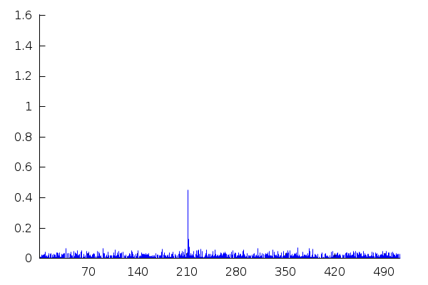
Let us add some white noise to a sinusoidal wave (of frequency w=211):
| (%i4) | y:map(lambda([z],float(sin(211·z)+random(float(%pi)))),x)$ |
| (%i5) | xy:makelist([x[k],y[k]],k,1,m+1)$ |
The result seems to be a completely random signal:
| (%i6) | wxplot2d([discrete,xy]); |
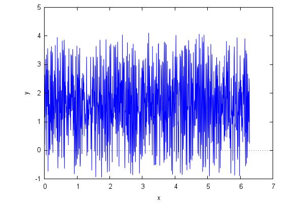
However, a frequency analysis (using the fast Fourier transform) reveals that inside the signal there is a regular, periodic wave of frequency... about w=211!
| (%i7) | with_stdout("/dev/null",load(fft))$ |
| (%i8) | z:map(abs,real_fft(y))$ |
| (%i9) | length(z); |
| (%i10) |
wxdraw2d(points_joined=impulses,line_width=1,color="blue",points(z), axis_top=false,axis_right=false,xtics=70); |
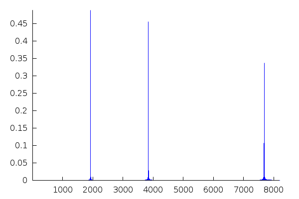
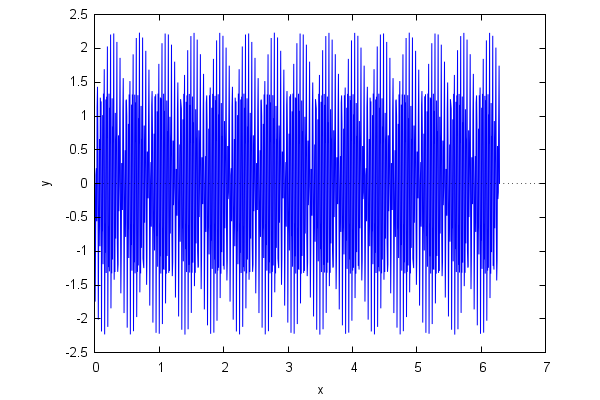
Now, we superimpose three rapidly oscillating signals of frequencies w0=1920, 2w0 and 4w0:
| (%i11) | x:float(makelist(2·%pi·j/m,j,0,m))$ |
| (%i12) | y:map(lambda([t],float(sin(1920·t)+sin(3840·t)+sin(7680·t))),x)$ |
| (%i13) | xy:makelist([x[k],y[k]],k,1,m+1)$ |
| (%i14) | wxplot2d([discrete,xy]); |
And repeat the procedure:
| (%i15) | u:map(abs,real_fft(y))$ |
| (%i16) |
wxdraw2d(points_joined=impulses,line_width=1,color="blue",points(u), axis_top=false,axis_right=false,dimensions = [700,300]); |
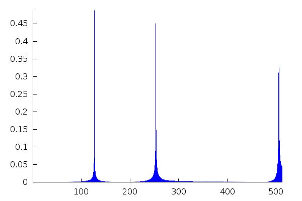
The three peaks are identified, with their relative separation, but their locations are displaced. This is due to the fact that the list u only contains 513 values (1024/2+1). To put the frequencies in their absolute abcissas, we must sample above the highest frequency:
| (%i17) | m:2^14−1$ |
| (%i18) | x:float(makelist(2·%pi·j/m,j,0,m))$ |
| (%i19) | y:map(lambda([t],float(sin(1920·t)+sin(3840·t)+sin(7680·t))),x)$ |
| (%i20) | xy:makelist([x[k],y[k]],k,1,m+1)$ |
| (%i21) | u:map(abs,real_fft(y))$ |
| (%i22) |
wxdraw2d(points_joined=impulses,line_width=1,color="blue",points(u), axis_top=false,axis_right=false,xtics=1000); |